Wildfire Smoke is Choking Seattle: visualizing using Altair
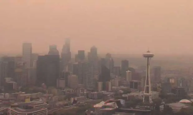 Image credit: MyNorthwest
Last week was tough for everyone in Seattle because of the bad air quality. Sadly, it was nothing compared to what we are going through this week. The Air Quality Index (AQI) reached well above 150 since Monday, which is roughly equal to “smoking seven cigarettes in a day.” The hazardous smoke is attributed to the surrounding massive wildfires, and the onshore winds to the rescue are expected to arrive first in the Wednesday evening.
Here is the experimental smoke forecast from NWS’ tweet on Tuesday:
Another round of #smoke from the wildfires in north central Washington and British Columbia is expected to impact the area this afternoon. This will keep smoke thick, at least through Wednesday. Smoke conditions at: https://t.co/cgLa9sAQBQ #WAwx pic.twitter.com/cgJHU5SS7u
— NWS Seattle (@NWSSeattle) August 21, 2018
News articles seem to be obsessed with the AQI number. When I tried plotting out the AQI levels in Seattle in the past week, I realized that the AQI is unitless, but the data I found has a typical aerosol measurement unit $\mu g/m^{3}$. So I dived deeper to find out more details about AQI, which I’d like to explain below.
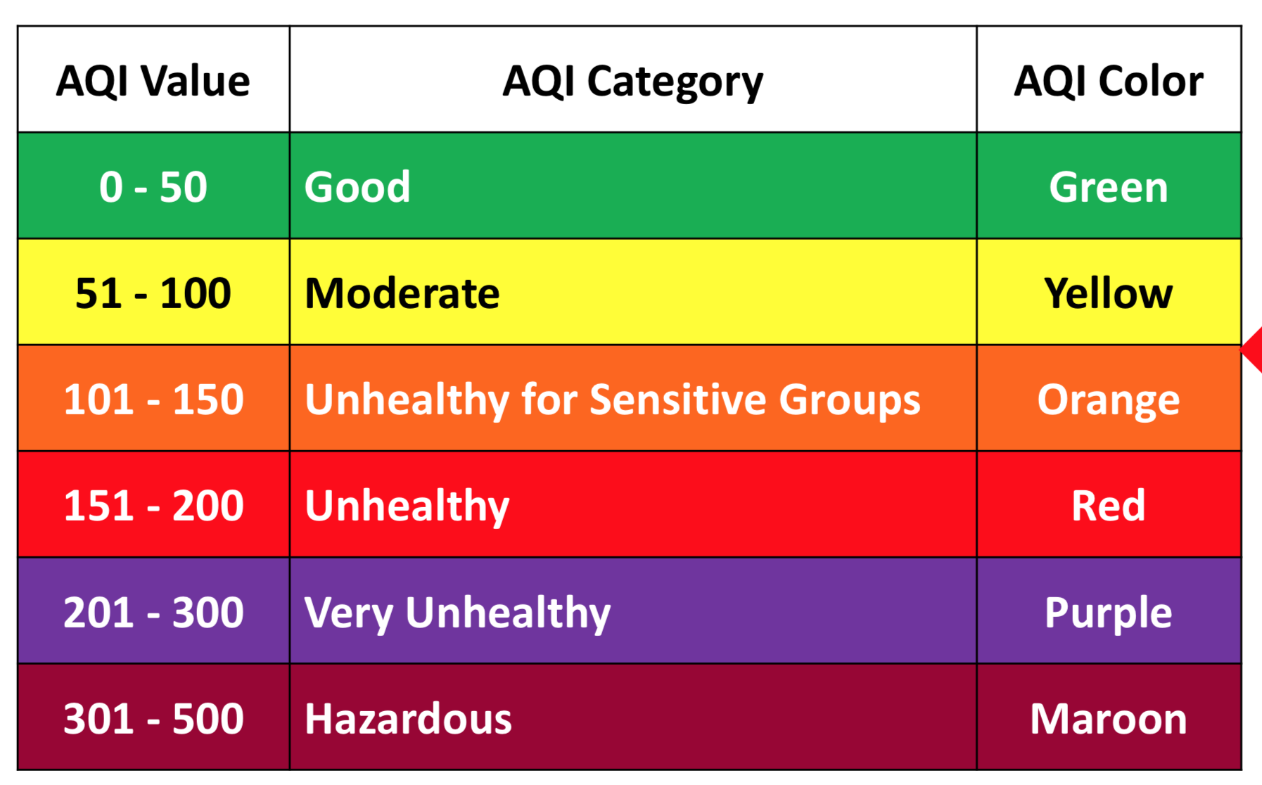
According to the EPA website, the AQI focuses on health effects, not strictly bounded to particle concentration. An AQI value of 100 corresponds to the national air quality standard for that pollutant, and EPA currently published AQI for four pollutants, ground level ozone, particle pollution, carbon monoxide, and sulfur dioxide. The number we saw in the news articles is for the particle pollution, specifically the PM2.5. Because the AQI 100 depends on the national standard, the AQI scale varies between countries and the regulatory agencies. Here is the current scale published by EPA:
However, the conversion between AQI and particle concentration is not linear. It is also not clear to me, what the averaging period of the reported AQI number is. After some googling, I found a chart published by EPA, but the conversion is based on the 24-hr average of particle concentration.
The station-based PM2.5 data is harder to find than I expected. Kudos to the Puget Sound Clean Air Agency for providing a fantastic online graphing tool and the downloadable data. Below I plotted the PM2.5 concentration in the past 10 days using Altair, a declarative statistical visualization library for Python, based on Vega and Vega-Lite.
Last Wednesday, the 24hrs-averaged PM2.5 concentration reached 95.4 $\mu g/m^{3}$, which is at the Unhealthy level. Yesterday the PM2.5 peaked at 154.9 $\mu g/m^{3}$, which is classified Very Unhealthy. Fortunately, the index seems to be declining in the past 24 hours.
Walk-through of the plot:
Clean up the dataframe: Altair takes in dataframes as data source. I changed the dtypes and the name of my two columns. One limitation is that Altair doesn’t recognize the index. So anything you want to plot need to be in columns (use reset_index)
Define the AQI levels as a dataframe
source, set the legend and corresponding colors and plot the rectangles using:alt.Chart(source).mark_rect()The line plot of PM2.5 with vertical line and circle while mouse hovering is composed of five elements (or layers): selectors, rule, line, point and text. This is adapted from one of the examples in the Altair gallery.
Combine the line plot and the rectengle, simply
(rect+layer).configure_axis(grid=False)
To my knowledge, the interactive plots you’ve seen on the Internet mostly involve javascript. Altair is no exception. It’s a wrapper that translates your python commands to Vega-lite/Vega-readable json objects. I really like the idea of “visualization grammar” that divides visualization into several building blocks. Vega/Vega-lite can take json objects and create rich interactive visualizations. I’ve been following Altair for quite a while, but only recently I decided to give it a spin. It’s my first plot using Altair. I’ll share more thoughts about Altair in future posts.
Yu Cheng 鄭嵎
Sustainability Data Scientist
Passionate about leveraging my past experience to make positive impacts on the planet. Well, raising two wonderful children heartfully is a good start.