Remove model drift using control run simulations
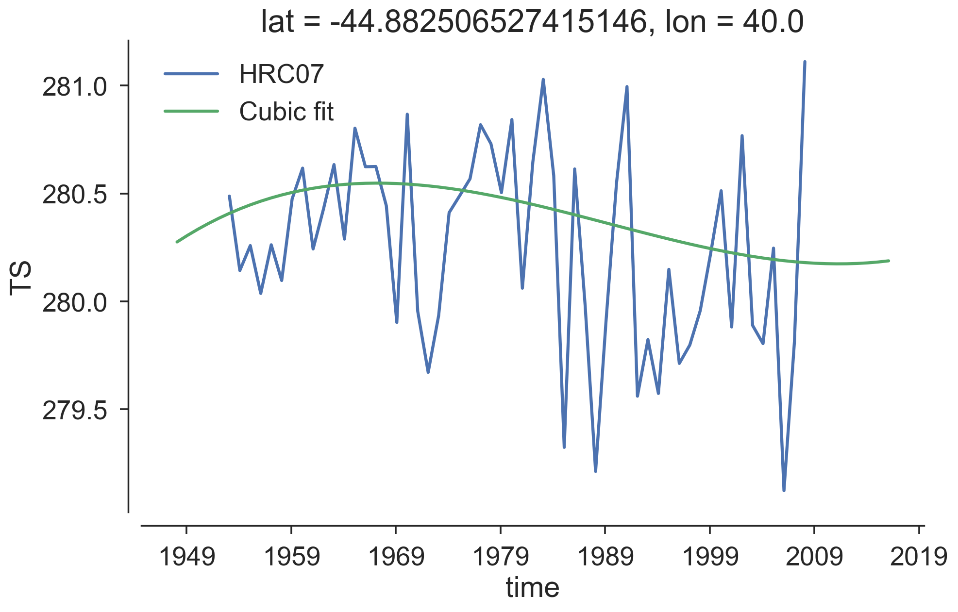
Recently, I’ve been trying to remove model drift from my high-resolution CCSM 20th century climate change simulation. The model drift is estimated using the two companion control runs, HRC08 and HRC09. All three runs were spun up from a similar initial condition, with CO2 held fixed in year 2000 level. Following Gupta et al., [2013]1, we tried to identify the model drift by fitting a cubic polynomial to the full record of control runs (nearly 70 years). The drift is then removed from the 20th-century climate change simulation. One thing is worth pointing out, this climate change run did not start from a pre-industrial level of CO2, but a year 2000 level forcing. Some variables, including the global mean sea surface temperature, may have lingering effect of higher CO2 level that takes few decades to reach the new equilibrium.
Below, I’d like to document my experience of cubic fitting the surface temperature (TS) locally at each grid point. Removing these drifts from the TS in the climate change run yields the de-drifted TS dataset. This post highlights several packages I’ve been using most frequently, including numpy, xarray and cartopy.
f1 = './data/TS.ens.all.nc'
ds1 = xarray.open_dataset(f1, decode_times=True, chunks={'lat':200,'lon':200})
TS_annual=ds1.TS.resample('12MS',dim='time')
These lines load in a NetCDF file with 69 years of monthly mean TS (time: 69, lat: 384, lon: 576) in (200x200) chunks. The chunk is the built-in support of Dask in Xarray. Xarray is a very powerful package. It attempts to extend the labeled data power of Pandas to the multi-dimensional datasets that we often work on in geophysical sciences.
import matplotlib.dates as dates
from numpy.polynomial.polynomial import polyval,polyfit
import xarray
def driftfit(arr):
    stacked = arr.stack(loc=('lat', 'lon'))
    timenum=dates.date2num(stacked.time.to_index().to_pydatetime())
    regressions = polyfit(timenum, stacked, 3)
    drift_stacked= polyval(timenum,regressions)
    foo = xarray.DataArray(drift_stacked.T, coords=[stacked['time'], stacked['loc']], dims=['time', 'loc'],name=arr.name)
    arr_drift=foo.unstack('loc')
    return arr_drift
This is a function to fit a 3rd order polynomial to the 69-year surface temperature of each grid cell. It stacks locations of the input array using arr.stack(loc=('lat', 'lon')), and using numpy.polynomial.polynomial.polyfit to find the cubic fit of the local temperature time series over 69 years. The coefficients are then converted back to the polynomials using polyval(timenum,regressions). Next step is to generate a DataArray from numpy.array so that I can unstack the array correctly and keep the metadata from the input DataArray.
polyfit are created equal. The numpy.polyfit outputs the polynomial coefficients from the highest power, while the numpy.polynomial.polynomial.polyfit does the other way round. And so are the input order of their corresponding polyval.I then load in the climate change run and remove the cubic fit from it. Two functions lintrend and trendts are constructed similarly to driftfit, so I left out the details. The former output the coefficient of the first order polynomial (the slope), and the later output the trend time series.
ensfit=driftfit(TS_annual)

f2 = './data/TS.HRC07.all.nc'
ds2 = xarray.open_dataset(f2, decode_times=True, chunks={'lat':200,'lon':200})
TS_HRC07_annual=ds2.TS.resample('12MS',dim='time')
TS_HRC07_dedrift=TS_HRC07_annual-ensfit
trend_HRC07=lintrend(TS_HRC07_dedrift)
trendTS_HRC07=trendts(TS_HRC07_dedrift)
After removing the drift from each location, I plot out the linear trend map of TS for the HRC07 run using cartopy.
plt.figure(figsize=(13,5))
ax = plt.subplot(111, projection=ccrs.PlateCarree()) #ccrs.Mollweide()
mm = ax.pcolormesh(ds1.lon,
                   ds1.lat,
                   trend_HRC07*365*10,
                   vmin=-.5,
                   vmax=.5,
                   transform=ccrs.PlateCarree(),cmap=cmo.balance )
ax.set_global()
#ax.set_extent([-180, 180, -70, 70])
ax.coastlines();
cb=plt.colorbar(mm,ax=ax,fraction=0.046, pad=0.01)


#ax.set_xticks([0, 60, 120, 180, 240, 300, 360], crs=ccrs.PlateCarree())

ax.set_xticks([-180,-120,-60,0, 60, 120, 180], crs=ccrs.PlateCarree())
ax.set_yticks([-90, -60, -30, 0, 30, 60, 90], crs=ccrs.PlateCarree())
lon_formatter = LongitudeFormatter()
lat_formatter = LatitudeFormatter()
ax.xaxis.set_major_formatter(lon_formatter)
ax.yaxis.set_major_formatter(lat_formatter)


ax.set_title('dedrifted HRC07 Temperature linear trend ')
cb.set_label('degC/decade')

plt.show()
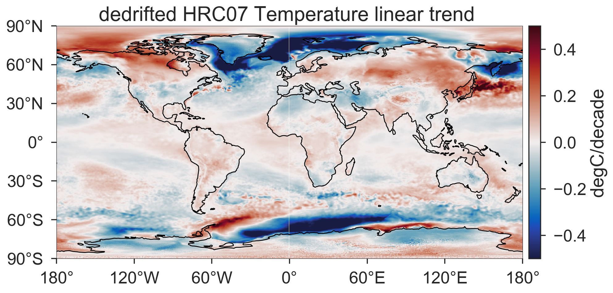
The cooling trends in the Agulhas System seem to contradict to what we anticipated and hence need a closer look. Note that this kind of trend and drift estimates highly depends on the chosen endpoints and available record lengths. In Gupta et al. [2013]1, drifts are estimated from multiple control runs of hundreds of years. For our high-resolution model, having multiple century-long control runs is a luxury. Maybe this technique is not applicable given the short record of our runs. Besides, estimating the drift locally may need to be justified.
Yu Cheng 鄭嵎
Sustainability Data Scientist
Passionate about leveraging my past experience to make positive impacts on the planet. Well, raising two wonderful children heartfully is a good start.